

A neural network written in Python to solve XOR problem.
The dimensions of this neural network can be changed dynamically. For XOR problem it is sufficient to have 2 neurons in the input layer, 10 neurons in the hidden layer, and 2 neurons in the output layer (classes ‘0’ and ‘1’). Dimensions are adjusted by this line of code:
# two input neurons, one hidden layer with 10 neurons, last layer with 2 output neurons
NN_dimensions = [2, 10, 2]

# a - number of inputs, Ln - number of neurons in hidden layers
NN_dimensions = [a, L1, L2, ..., Ln]
In this code example, the number of iterations is fixed, and the learning rate is fixed as well. This project was made with one purpose: delving into the essence of neural networks, that is, math.
Weight notation, where (n) – layer index, i – neuron index, j – weight index:
Bias value, where (n) – layer index, i – neuron index:
The weighted sum value z of a neuron, where (n) – layer index, i – neuron index:
The activation value a of a neuron, where (n) – layer index, i – neuron index:
The predicted output for class i, where i is the index of neuron in the last (output) layer:
The expected output for class i, where i is the index of neuron in the last (output) layer:
The cost function of the whole neural network:
The learning process is, in simple words, many repetitions of “moving” forward and calculating activation values, then going backward and adjusting weights and biases based on that. For the forward propagation, we use functions of weighted sum, activation and square error. For backpropagation we have to find derivatives of square error with respect to activation, then derivative of activation with respect to weighted sum, and lastly derivative of weighted sum with respect to weight.
As mentioned before, it is necessary to calculate the sum values z for every neuron in every hidden layer. We use the formula as follows (M – number of neurons in the previous layer):
The activation function of every neuron in this neural network is sigmoid. It is calculated as follows:
The cost function used here is slightly different from MSE (Mean Square Error). Instead of taking the mean of all square errors, we take 1/2. This is done in order for the derivative to be a bit simpler. MSE (or C) is calculated as follows:
In order to calculate the gradient for each weight we have to calculate the partial derivative of cost with respect to that weight. I find it easier to think of this process as “finding the path that leads from cost to that weight“.
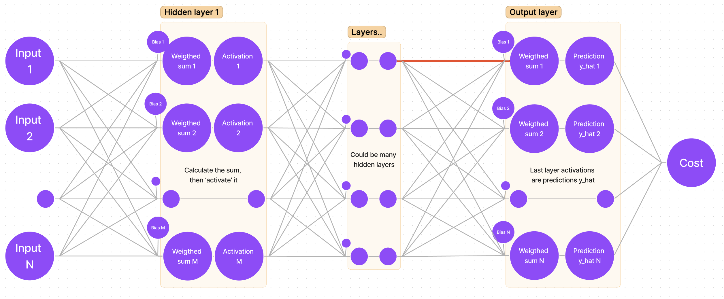
If we sketch our neural network, we get a generalized graph:

First things first, we want to adjust the weights for the output (last) layer (remember, we are starting from “the end”). It means that we are looking for:
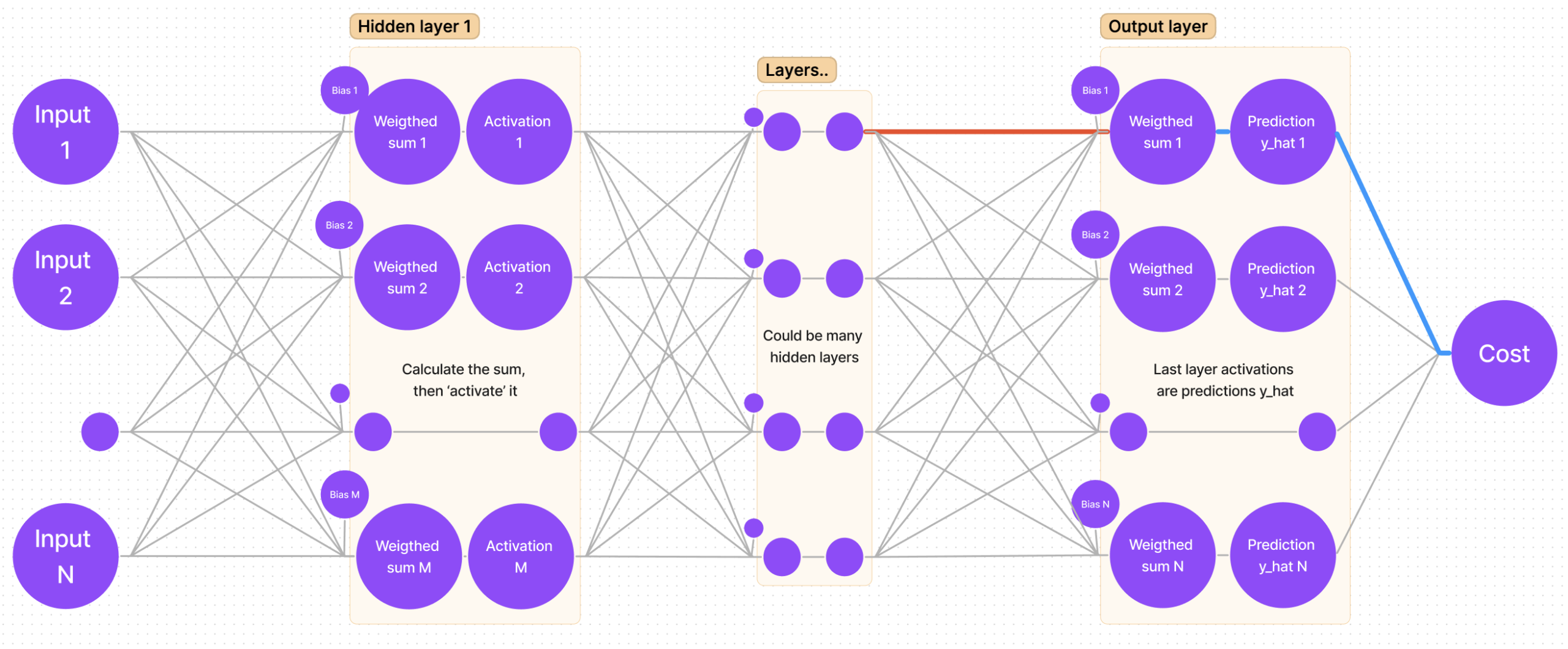
Suppose we are looking for the gradient for the first weight of the first neuron. In the sketch, that weight is marked with a bold red line:

I myself use an intuitive way for finding the derivative: follow the path from the cost function to that weight you are looking for (bold blue lines):

It is clear that we have to “traverse” through cost-y_hat, then y_hat-sum, and lastly sum-weight. That’s the same as saying: find the partial derivative of cost with respect to y_hat, then find the partial derivative of y_hat with respect to sum, and finally the partial derivative of sum with respect to weight.
So, if we are calculating gradients for the last layer n, by following the chain rule, we get the following equation:
In order to solve it, let’s first find each derivative:
Putting it all back together, we get the full gradient:
If we want to adjust the bias, then the partial derivative of sum with respect to bias is 1; we get:
That’s it! Having found the gradient for each weight in the output layer, we can use it to adjust the weights:
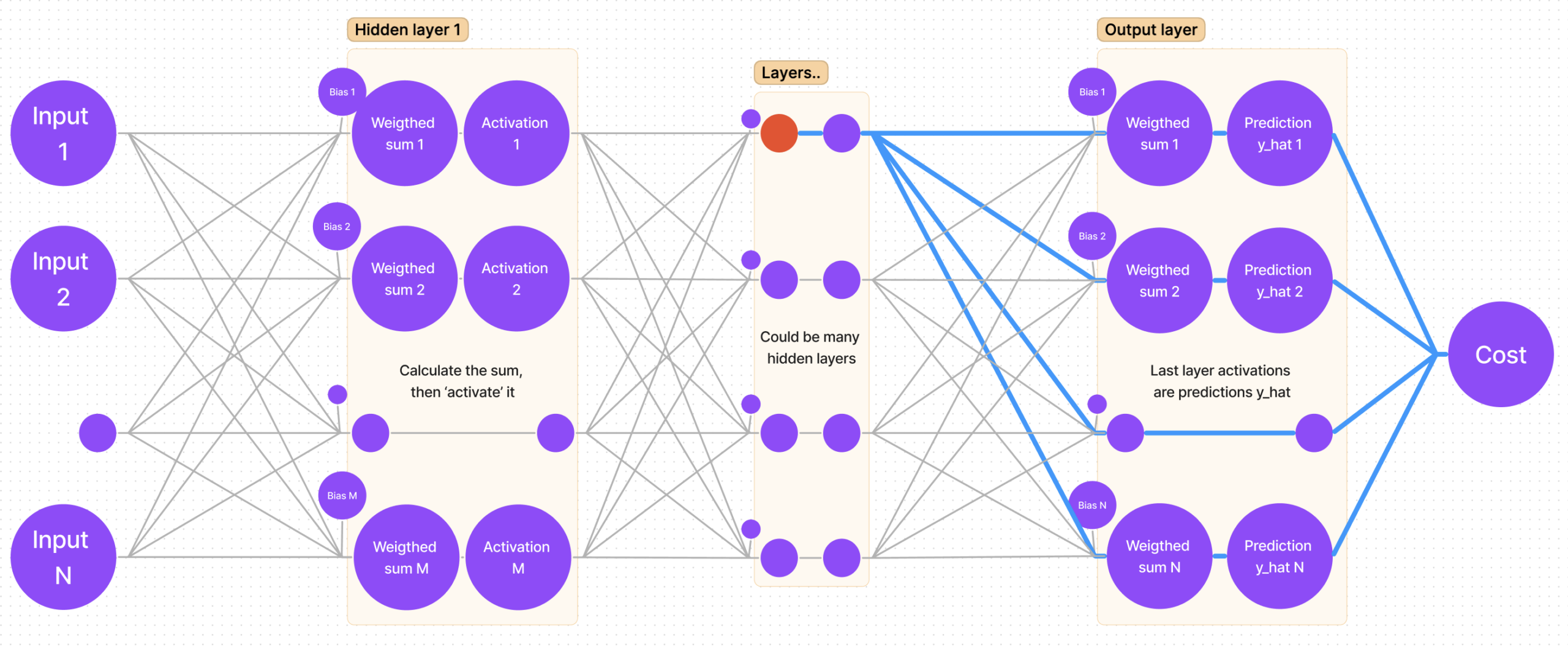
Graphical visualization of the chain rule for hidden layers
Now the harder part is calculating the gradient for hidden layers. Luckily, there is a pattern for calculating the derivatives, as some of them repeat themselves in different layers’ equations. To acknowledge that pattern, we must not calculate the derivative of cost with respect to weight, but find the partial derivative of cost with respect to sum (this way we will be able to save that derivative value and use it later).
Let’s once again mark the sum of a hidden layer with the color red:

Now let’s find all paths from cost to that sum:

It is clear that there’s more than one path, but that’s quite easy to account for – the calculation is done by adding all partial derivatives that we get “traversing each path”!
Mathematical approach and applying chain rule for hidden layers
There’s one unresolved question: why take the derivatives of cost with respect to sum and not with respect to weight? As we will soon find out, there is a pattern: derivatives repeat themselves, hence calculating and saving derivatives as we move from the outer layer (BACK propagation) to ‘front’ enables us to reuse the values (note: remember what I said about “traversing all paths” and adding them up? That’s where the summation sign comes from; M – number of neurons in the next (n+1) layer):
Note how the last derivative is constant in terms of k (that value is the same for every member in the summation), so we can put it before the summation sign. Also note, that we have two partial derivatives that can be rewritten as one:
We get:
Calculate derivatives that we can find:
Plug the values back into the equation:
Notice how for the cost derivative with respect to sum in layer n we have to use the cost derivative with respect to sum in layer (n+1). That’s the most important part of making the code work – saving the derivatives.
Now we know everything we need to know to use the gradient descent algorithm. Let’s sum up really quickly and get to coding!
As the most important part of the program is saving partial derivatives of cost with respect to each layer’s sum, let’s write it in a nice and concise way.
Derivative for the last layer:
The general expression for any hidden layer:
Once we have calculated all derivatives, we can adjust the weights by calculating the full gradient and subtracting it from that weight. Here we have two general formulas. First one for adjusting any weight:
And a second one for adjusting the bias value (optionally: add a0 = 1 to your activations array and use the previous formula):
Finally, we get a really neat and clean weight (accordingly bias) adjustment equation:
Leave a Reply